Ymarferol 2: Machine Translation
1 Using Machine Translation Models
1.1 The transformer architecture
MarianMTModel( (model): MarianModel( (shared): Embedding(54395, 512, padding_idx=54394) (encoder): MarianEncoder( (embed_tokens): Embedding(54395, 512, padding_idx=54394) (embed_positions): MarianSinusoidalPositionalEmbedding(512, 512) (layers): ModuleList( (0-5): 6 x MarianEncoderLayer( (self_attn): MarianAttention( (k_proj): Linear(in_features=512, out_features=512, bias=True) (v_proj): Linear(in_features=512, out_features=512, bias=True) (q_proj): Linear(in_features=512, out_features=512, bias=True) (out_proj): Linear(in_features=512, out_features=512, bias=True) ) (self_attn_layer_norm): LayerNorm((512,), eps=1e-05, elementwise_affine=True) (activation_fn): SiLU() (fc1): Linear(in_features=512, out_features=2048, bias=True) (fc2): Linear(in_features=2048, out_features=512, bias=True) (final_layer_norm): LayerNorm((512,), eps=1e-05, elementwise_affine=True) ) ) ) (decoder): MarianDecoder( (embed_tokens): Embedding(54395, 512, padding_idx=54394) (embed_positions): MarianSinusoidalPositionalEmbedding(512, 512) (layers): ModuleList( (0-5): 6 x MarianDecoderLayer( (self_attn): MarianAttention( (k_proj): Linear(in_features=512, out_features=512, bias=True) (v_proj): Linear(in_features=512, out_features=512, bias=True) (q_proj): Linear(in_features=512, out_features=512, bias=True) (out_proj): Linear(in_features=512, out_features=512, bias=True) ) (activation_fn): SiLU() (self_attn_layer_norm): LayerNorm((512,), eps=1e-05, elementwise_affine=True) (encoder_attn): MarianAttention( (k_proj): Linear(in_features=512, out_features=512, bias=True) (v_proj): Linear(in_features=512, out_features=512, bias=True) (q_proj): Linear(in_features=512, out_features=512, bias=True) (out_proj): Linear(in_features=512, out_features=512, bias=True) ) (encoder_attn_layer_norm): LayerNorm((512,), eps=1e-05, elementwise_affine=True) (fc1): Linear(in_features=512, out_features=2048, bias=True) (fc2): Linear(in_features=2048, out_features=512, bias=True) (final_layer_norm): LayerNorm((512,), eps=1e-05, elementwise_affine=True) ) ) ) ) (lm_head): Linear(in_features=512, out_features=54395, bias=False))This model is divided in four parts, first comes the embedding layer. It’s first layer is a shared layer, which means it is used both by the encoder and the decoder. Its role is to turn the token into vectors and the vectors back to tokens (which are then turned back to real words). This embedding layer can recognise 54395 different tokens and turns them into 512 ($2^9$) dimensions-long vectors. The Padding vector is in the 54394th (last) postition.
Then comes the encoder. It starts with the same layer as describe above followed by a positional embedding layer, in order to make sure the transformer architecture gets a sense of which word is in which position in the sequence, which they don’t do like RNN like LSTM and GRU. It uses sinusoidal functions to create the “positional matrix” whose values are added to the embedded words vectors of the sequence. After this comes the self-attentions layers, six of them.
The decoder follows a similar pattern except that it also include a cross-attention layer. The model ends with a language model head, which converts the vectors in tokens, similarly to the way a simpler NN architecture would end with a layer using the softmax activation function to transfor the last vector produced by the network in a one dimentional categorical value.
1.2 Translation with a multilingual model
To enable translation from several different languages we add a language tag in the beginning of the sentence. Note that only the Welsh model gives a correct translation. In Breton it translates to “This is famous!” and in Cornish to “It was the biggest proktoryon”, whatever that means.
src_txt= [f'>>{lid}<< This is a great practical!' for lid in ['br', 'cy', "kw"]]
['Brudet eo an dra-se !', 'Mae hyn yn ymarferol iawn!', "Yth esa'n brassa proktoryon!"]
2 Models Evaluation
2.1 modifications
In this sections we will examine the modifications I made to the base colab file.
2.1.1 Data preparation
As I extracted a parallel corpus (Breton and French litterary translations) for the previous practical (the corpus come from this wiki on comparative stylistic). I thought of using its 128 sentences as my testing set for a Breton-French translation model:
ds_trgt_lang=datasets.load_dataset('gsarti/flores_101', trgt_lang)
with open("/content/corpus_content.json") as f:    parallel_corpus = json.load(f)
ds_src_lang = [sent["br"] for sent in parallel_corpus]ds_trgt_lang = [sent["fr"] for sent in parallel_corpus]
2.1.2 Model
I looked in HuggingFace for a French-Breton model and found lgrobol/m2m100_418M_br_fr, Loïc Grobol’s fine tuned version of facebook/m2m100_418M. Here are the most meaningful modifications:
First, we import the model, tokenazer and testing everything works by translating the first sentence.
model_name = "lgrobol/m2m100_418M_br_fr"
# import M2M tokenizer and modelfrom transformers import M2M100ForConditionalGeneration, M2M100Tokenizermodel = M2M100ForConditionalGeneration.from_pretrained(model_name)
tokenizer = M2M100Tokenizer.from_pretrained(model_name)
tokenizer.src_lang = "br"tokenized_source = tokenizer(ds_src_lang[0], return_tensors="pt", padding=True)
generated_tokens = model.generate(**tokenized_source, forced_bos_token_id=tokenizer.get_lang_id("fr"))
tokenized_translated = tokenizer.batch_decode(generated_tokens, skip_special_tokens=True)print(ds_src_lang[0])# A dra sur n'en doa ket gellet Doue faziañ ha kuzhet e oa ster an istor-se tu bennak met ne oa ket en addisplegoù.print(tokenized_translated)# C'est certainement que Dieu n'avait pas pu faire faim et que l'histoire n'avait pas été cachée, mais qu'elle n'était pas dans les interprétations.
# import progress bar for our own for loops.from tqdm import tqdm
# translate all the sentencesprint("Producing machine translations.....")for i, d in enumerate(tqdm(ds_src_lang)): src_txts.append(d)
translated = model.generate(**tokenizer(d, return_tensors="pt", padding=True), forced_bos_token_id=tokenizer.get_lang_id("fr"))
tokenized_translated = tokenizer.batch_decode(translated, skip_special_tokens=True)[0] hyp_txts.append(tokenized_translated)2.2 Results
Here are examples of translated sentences.
“Les animaux derrière la cire réchauffent les maîtres.” (cire means wax) translated from: “Al loened a-dreñv ar speurenn o tommañ ar vistri;” (The animals behind the wall warming the masters.). Here the word for “wall” is translated by “wax”…
But some translations are actually good, possibly better than the original depending on the context. The following is the translation for this sentence:
“Tout le dimanche fut un défilé d’insurrection à la maison de Gourvennec.”
It properly translates the name and come up with an idea of “insurrection” that is not present in the breton source…
We can finally analyze the result. The BLEU score is 14,5. Which is signifantly improvable.
{'score': 14.519707899178815, 'counts': [1553, 630, 294, 150], 'totals': [3198, 3070, 2942, 2814], 'precisions': [48.561601000625394, 20.521172638436482, 9.99320190346703, 5.330490405117271], 'bp': 0.9565686202237099, 'sys_len': 3198, 'ref_len': 3340}3 Training and Fine-tuning a MT Engine
Here is the orignial value of the Welsh-English model:
{'score': 11.511182155223498, 'counts': [10364, 3892, 1757, 820], 'totals': [23621, 22624, 21628, 20632], 'precisions': [43.876211845391815, 17.202970297029704, 8.123728500092472, 3.9744086855370298], 'bp': 0.9213079194653137, 'sys_len': 23621, 'ref_len': 25557}Here is the fine tuned results:
{'score': 13.268464073731995, 'counts': [11206, 4427, 2064, 1005], 'totals': [24933, 23936, 22939, 21942], 'precisions': [44.944451129025786, 18.49515374331551, 8.997776712149614, 4.580257041290675], 'bp': 0.9752835082550481, 'sys_len': 24933, 'ref_len': 25557}It is a staggering to see how far this improvement is in comparison to the 30.355800 BLEU score clamed against the testing set from the memory translation. This informs us of two facts:
- Fine-tuning works especially well if the goal is to use the model in a similar context to the one of the data that were used in the fine tuning training set. And conversely, the fine-tuning bring little benefits in a less resrticted context, which underlines the importance of building larger “generalist” models and gathering bigger data sets to train them.
- It is really important to have a testing set as rich as possible to ensure that our testing results are not misleading when trying to build general-purpose models.
Next, we will try to improve these results.
3.1 Better data and hyperparameters
I tried to load as many parallel sentences as possible for this new training. I ended up with a training set of 600 244 sentences and a testing and a validation set of 75 030 and 75 031 pairs respectively. It took an hour and a half to retrieve the sentences from the translation memory, but the training never kicked off because I tried using a TPU instead of a GPU. So for the next attempts, I restricted the number of MTX files to 120, where as it was 100 only in the original one. In order not to run out of memory, I used a A100 GPU for the runtime. Here are my modifications regarding the model’s hyperparameters:
args = Seq2SeqTrainingArguments( training_dir, evaluation_strategy = "epoch", learning_rate=2e-4, per_device_train_batch_size=batch_size, per_device_eval_batch_size=batch_size, weight_decay=0.05, save_total_limit=3, num_train_epochs=5, predict_with_generate=True)First, I increased the learning rate a bit, from 2e-5 to 2e-4, as well as the weight decay to 0.05. This had a positive impact because, at the end of the first epoch, the BLEU score against the testing dataset was of 39.926900 and not 30.355800 as in the initial fine tuning, unless this improvement was because of the high quality of the additional 20 MTX files that where included in the training (but also the testing) data set. This second hypothesis is unlikelly because it is hard to imaging a 30% improvement when adding only 20% more data, especially when taking in consideration the Zipf law and the Heap’s law. Adding more data should help, but not so much, so we can be confident that an increased learning rate helped in this case. Secondly, I increased the number of epochs from 1 to 5. This increases the time of training significantly, but also the results optained.
3.2 Training data and graphs
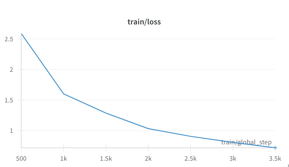 Figure 1. The loss function over the training set.
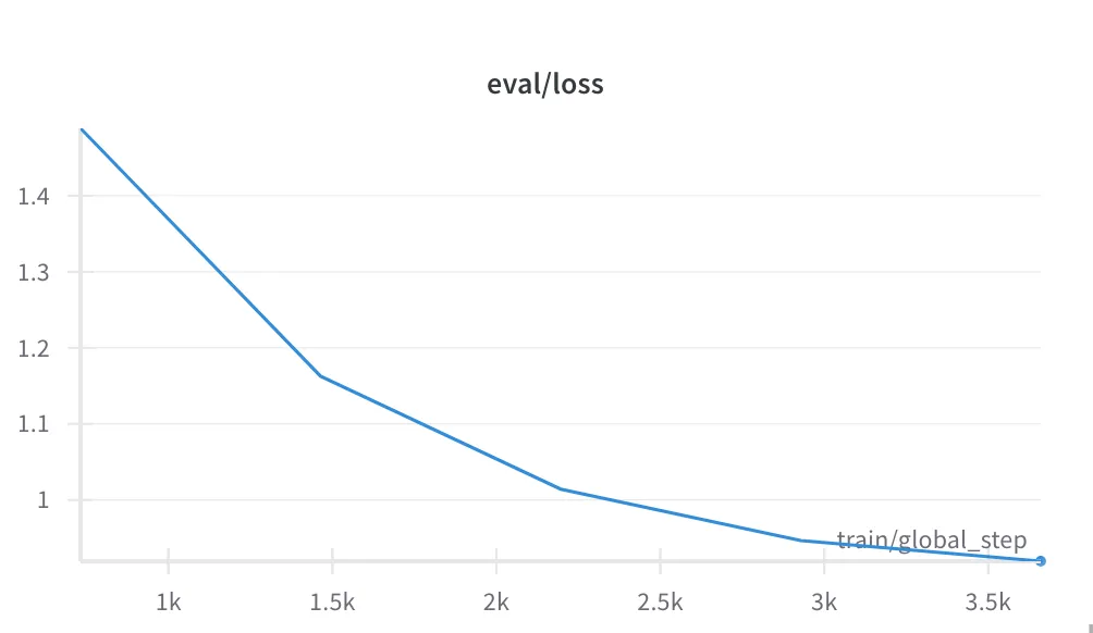 Figure 2. The loss function over the evaluation data set. As we can see, there was no overfitting during the process.
This table shows the minutes of the training process.
Figure 2. The loss function over the evaluation data set. As we can see, there was no overfitting during the process.
This table shows the minutes of the training process.
| Epoch | Training Loss | Validation Loss | Bleu | Gen Len |
|---|---|---|---|---|
| 1 | 2.588400 | 1.488559 | 39.926900 | 26.122100 |
| 2 | 1.602400 | 1.162717 | 48.640400 | 25.739000 |
| 3 | 1.033800 | 1.014269 | 52.045500 | 26.224600 |
| 4 | 0.907500 | 0.946714 | 54.258300 | 26.136200 |
| 5 | 0.720300 | 0.919511 | 55.276300 | 26.243800 |
| As we can see, the BLEU score is really close to the state of the art. But let us see how the model performs agains a different, more diverse, testing dataset. |
3.3 Results against the flores testing dataset
{'score': 17.93191854470908, 'counts': [12455, 5685, 2986, 1627], 'totals': [25210, 24213, 23216, 22219], 'precisions': [49.40499801666006, 23.479122785280634, 12.861819434872501, 7.322561771456861], 'bp': 0.9863299167155396, 'sys_len': 25210, 'ref_len': 25557}As we can see, there is indead an improvement, but nowhere as big as the one seen on the testing data set from the translation memory. This confirms the points made in the begining of this section.